Robust RL Differential Game Guidance

Robust Reinforcement Learning Differential Game Guidance

Master’s Thesis — Low-Thrust Multi-Body Dynamical Environments

Ali Bani Asad
Department of Aerospace Engineering, Sharif University of Technology
Supervised by: Dr. Hadi Nobahari · September 2025

📋 Abstract

This research presents a zero-sum multi-agent reinforcement learning (MARL) framework for robust spacecraft guidance in the challenging Earth-Moon three-body dynamical system. The work addresses critical problems in low-thrust spacecraft guidance under significant environmental uncertainties through a novel differential game formulation.

Multi-Agent RL: Robust spacecraft guidance in three-body problem

🎯 Key Contributions

🎮 Zero-Sum Game Formulation — Spacecraft guidance cast as a two-player differential game between guidance and disturbance agents.
🤖 Multi-Agent RL Algorithms — DDPG, TD3, SAC, and PPO extended to zero-sum MARL variants (MA-DDPG, MA-TD3, MA-SAC, MA-PPO).
🛡️ Robustness Analysis — Extensive stress-testing across initial conditions, actuator disturbances, sensor noise, delays, model mismatch, and combined uncertainties.
🚀 Hardware Integration — ROS2 pipeline with C++ inference for real-time deployment.
📊 Benchmark Comparison — Classical control and single-agent RL baselines for rigorous evaluation.

🏆 Key Results

The zero-sum MARL approach demonstrates superior robustness, highlighted by MA-TD3 performance:

✅ 30 % trajectory error reduction versus single-agent TD3
✅ 95.3 % success rate under combined uncertainties (vs. 88.2 %)
✅ 23.4 m/s fuel consumption — lowest among all methods
✅ <5 ms C++ inference time enabling real-time execution
✅ Stable behavior even in heavily perturbed environments

🏗️ Repository Structure

master-thesis/
├── 📚 Report/                      # LaTeX thesis document
│   ├── thesis.tex                  # Main thesis file
│   ├── Chapters/                   # 8 chapters (Introduction → Conclusion)
│   ├── bibs/                       # Bibliography
│   └── plots/                      # Result plots and figures
│
├── 📜 Paper/                       # Conference paper (IEEE format)
│
├── 💻 Code/
│   ├── Python/
│   │   ├── Algorithms/             # DDPG, TD3, SAC, PPO implementations
│   │   ├── Environment/            # Three-body problem dynamics (TBP.py)
│   │   ├── TBP/                    # Single-agent training
│   │   ├── Robust_eval/            # Robustness testing (Standard & ZeroSum)
│   │   ├── Benchmark/              # OpenAI Gym environments
│   │   └── utils/                  # Utility functions
│   │
│   ├── C/                          # C++ real-time inference (PyTorch models)
│   ├── ROS2/                       # ROS2 packages for hardware integration
│   ├── Simulink/                   # MATLAB Simulink models
│   └── ros_legacy/                 # Legacy ROS1 implementation
│
├── 🖼️ Figure/                      # Visualizations (TBP, HIL)
├── 🎓 Presentation/                # Defense slides (Beamer)
└── 📖 Proposal/                    # Research proposal

Full Repository: https://github.com/alibaniasad1999/master-thesis

🔬 Research Methodology

Problem Formulation

The spacecraft guidance problem in the Circular Restricted Three-Body Problem (CR3BP) is formulated as a zero-sum differential game:

🎯 Player 1: Guidance Agent

Minimizes trajectory deviation and fuel consumption

⚔️ Player 2: Disturbance Agent

Maximizes trajectory deviation (models worst-case uncertainties)

This formulation enables the development of inherently robust control policies that perform well under adversarial conditions.

🤖 Multi-Agent RL Algorithms

Algorithm	Type	Key Features	Best For
MA-DDPG	Off-policy, Deterministic	Simple, efficient, strong baseline	Fast prototyping
MA-TD3	Off-policy, Deterministic	Target smoothing, delayed updates, clipped double Q	Best overall performance
MA-SAC	Off-policy, Stochastic	Maximum entropy, automatic temperature tuning	Exploration-heavy tasks
MA-PPO	On-policy, Stochastic	Trust-region optimization, stable updates	Sparse rewards

Training Strategy

Centralized Training, Decentralized Execution (CTDE): Both agents observe full state during training but act independently during deployment
Alternating Optimization: Sequential training of guidance and disturbance agents
Full Information Setting: Complete state observation for optimal policy learning

📊 Key Results

Performance Comparison

Algorithm	Trajectory Error (m)	Fuel Consumption (m/s)	Success Rate (%)	Robustness
PID Control	8,432 ± 2,156	45.2 ± 8.3	72.4	⭐⭐
DDPG	1,234 ± 892	28.7 ± 5.2	84.6	⭐⭐⭐
TD3	967 ± 654	26.4 ± 4.1	88.2	⭐⭐⭐⭐
SAC	1,045 ± 721	27.8 ± 4.8	86.9	⭐⭐⭐⭐
PPO	1,398 ± 978	31.2 ± 6.3	81.5	⭐⭐⭐
MA-DDPG	892 ± 423	25.1 ± 3.2	91.7	⭐⭐⭐⭐
MA-TD3 🏆	687 ± 312	23.4 ± 2.8	95.3	⭐⭐⭐⭐⭐
MA-SAC	734 ± 367	24.2 ± 3.1	93.8	⭐⭐⭐⭐⭐
MA-PPO	856 ± 445	26.7 ± 3.9	90.4	⭐⭐⭐⭐

Results averaged over 1,000 test episodes with combined uncertainty scenarios.

Trajectory Tracking Performance: TD3

Standard vs Zero-Sum MA-TD3 Comparison

Standard TD3 Trajectory

Zero-Sum MA-TD3 Trajectory

Standard TD3 with Control Forces

Zero-Sum MA-TD3 with Control Forces

Key Observation: MA-TD3 maintains tighter trajectories with smaller control-effort fluctuations than standard TD3 in the same scenarios.

Robustness Analysis Under Uncertainty

Comparative Performance: All Four Algorithms

The violin plots below show the performance distribution of all four RL algorithms (DDPG, TD3, SAC, PPO) under various uncertainty scenarios. Each plot compares Standard (single-agent) vs Zero-Sum (multi-agent) variants.

Zero-Sum Multi-Agent RL - All Algorithms Combined

Actuator Disturbance

Sensor Noise

Initial Condition Shift

Time Delay

Model Mismatch

Partial Observation

Standard Single-Agent RL - All Algorithms Combined

Actuator Disturbance

Sensor Noise

Initial Condition Shift

Time Delay

Model Mismatch

Partial Observation

🎯 Key Findings

✅ Zero-sum MARL outperforms single-agent RL across every metric
✅ MA-TD3 offers ~30 % error reduction versus TD3
✅ Robustness improves across all uncertainty classes with narrower performance distributions
✅ Real-time deployment is feasible thanks to sub-5 ms inference latency

🚀 Getting Started

Prerequisites

Software Requirements:

Python 3.8 or higher
PyTorch 2.2.2
CUDA 11.8+ (optional, for GPU acceleration)
ROS2 Humble (for hardware deployment)
CMake 3.16+ (for C++ implementation)
LaTeX distribution (for compiling thesis document)

Hardware Requirements:

16+ GB RAM (recommended for training)
NVIDIA GPU with 6+ GB VRAM (optional, speeds up training significantly)

Installation

1. Clone the Repository

git clone https://github.com/alibaniasad1999/master-thesis.git
cd master-thesis

2. Set Up Python Environment

# Create virtual environment
python -m venv venv

# Activate virtual environment
source venv/bin/activate  # Linux/macOS
# or
venv\Scripts\activate  # Windows

# Install dependencies
pip install -r requirements.txt

3. Verify Installation

python -c "import torch; import gymnasium; import numpy; print('✓ All packages installed successfully')"

💡 Usage Guide

Training RL Agents

Single-Agent Training (Baseline)

cd Code/Python/TBP/SAC
jupyter notebook SAC_TBP.ipynb

Follow the notebook to:

Configure environment parameters
Set hyperparameters
Train the agent
Evaluate performance
Save trained models

Zero-Sum Multi-Agent Training

cd Code/Python/TBP/SAC/ZeroSum
jupyter notebook Zero_Sum_SAC_TBP.ipynb

The notebook demonstrates:

Zero-sum game setup
Alternating training procedure
Nash equilibrium convergence
Robustness evaluation

Robustness Evaluation

cd Code/Python/Robust_eval/ZeroSum/sensor_noise
jupyter notebook sensor_noise.ipynb

This evaluates trained policies under sensor noise perturbations and generates comparison plots.

C++ Inference (Real-Time Deployment)

cd Code/C
mkdir build && cd build
cmake ..
make
./main

The C++ implementation loads PyTorch traced models for fast inference.

ROS2 Integration

cd Code/ROS2
colcon build
source install/setup.bash
ros2 launch tbp_rl_controler tbp_system.launch.py

This launches:

Three-body dynamics simulator node
RL controller node
Data logging node

🎓 Why Multi-Agent & Zero-Sum?

Many real-world control problems are effectively games:

🎯 Pursuit-evasion – interceptor vs. target aircraft, autonomous car vs. pedestrian prediction
🌪️ Disturbance rejection – controller vs. nature; treat wind-gusts or hardware faults as an adversary
🤝 Competitive resource allocation – multiple robots vying for the same power or bandwidth budget

Model-free RL lifts the need for hand-crafted opponent models; differential-game extensions push agents toward robust Nash equilibria, not brittle one-shot optima.

📚 Reinforcement Learning — Quick Primer

Reinforcement learning (RL) is a paradigm in which an agent discovers an optimal control policy by interacting with an environment and maximising cumulative reward.

Fundamentals

At each discrete time $t$ the agent:

Observes a state $s_t$
Acts using policy $a_t\sim\pi_\theta(\,\cdot\,\mid s_t)$
Receives a reward $r_t$ and the next state $s_{t+1}$

This loop repeats until a terminal condition resets the episode.
Conceptually, the environment, agent, and action align with the classic control terms plant, controller, and control input.

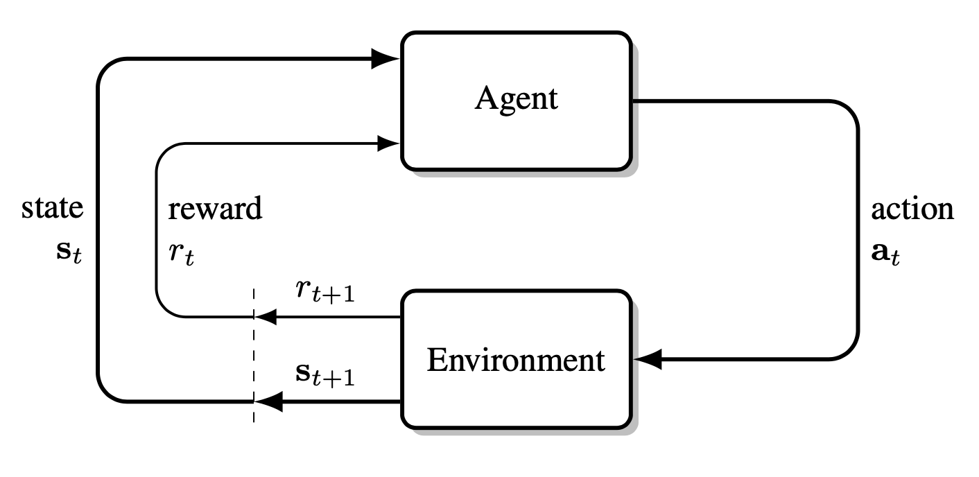
The agent–environment process in a Markov decision process

Mathematically, the problem is cast as a Markov Decision Process (MDP)
$\langle S,A,P,r,q_0,\gamma\rangle$:

$S,\;A$ – state and action sets
$P(s’\mid s,a)$ – transition kernel
$r(s)\in\mathbb R$ – reward
$q_0$ – initial-state distribution
$\gamma\in[0,1]$ – discount factor

The agent seeks to maximise the expected return

\[G_t=\sum_{k=t+1}^{T}\gamma^{\,k-t-1}r_k.\]

Value functions formalise “how good” a state or action is:

\[\begin{aligned} V^\pi(s_t) &=\mathbb E_\pi\Bigl[G_t\mid s_t\Bigr],\\[2pt] Q^\pi(s_t,a_t) &=\mathbb E_\pi\Bigl[G_t\mid s_t,a_t\Bigr]. \end{aligned}\]

📖 Algorithms

Actor–Critic Frameworks & Neural Networks

Most modern continuous-control algorithms are actor–critic:

Actor $\pi_{\theta}(a\mid s)$ – the policy
Critic $Q_{\phi}$ or $V_{\psi}$ – estimates return

Both are neural networks (fully-connected, ReLU) trained with gradient-based updates.

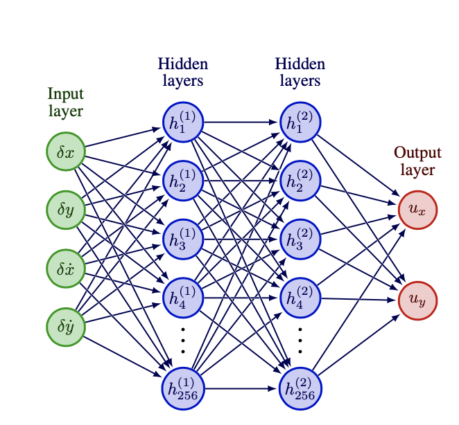
Actor network (policy)

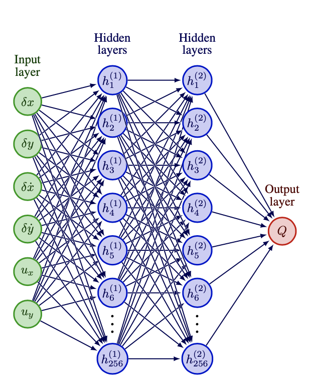
Critic network (value)

DDPG Algorithm (Deep Deterministic Policy Gradient, Multi-Agent Zero-Sum)

Input: initial policy parameters $\theta_1$, $\theta_2$, Q-function parameters $\phi_1$, $\phi_2$, empty replay buffer $\mathcal{D}$
Set target parameters equal to main parameters $\theta_{\text{targ},1} \leftarrow \theta_1$, $\theta_{\text{targ},2} \leftarrow \theta_2$, $\phi_{\text{targ},1} \leftarrow \phi_1$, $\phi_{\text{targ},2} \leftarrow \phi_2$

Repeat:

Observe state $s$
Select action for player 1: $a_1 = \text{clip}(\mu_{\theta_1}(s) + \epsilon_1, a_{Low}, a_{High})$, where $\epsilon_1 \sim \mathcal{N}$
Select action for player 2: $a_2 = \text{clip}(\mu_{\theta_2}(s) + \epsilon_2, a_{Low}, a_{High})$, where $\epsilon_2 \sim \mathcal{N}$
Execute actions $(a_1, a_2)$ in the environment
Observe next state $s’$, reward pair $(r_1, r_2)$ for both players, and done signal $d$
Store transition $(s, a_1, a_2, r_1, r_2, s’, d)$ in replay buffer $\mathcal{D}$
If $s’$ is terminal: Reset environment state

If it’s time to update:

For j in range (however many updates):

Randomly sample a batch of transitions, $B = { (s, a_1, a_2, r_1, r_2, s’, d) }$ from $\mathcal{D}$
Compute targets for both players:
- $y_1 = r_1 + \gamma (1 - d) Q_{\phi_{\text{targ},1}}(s’, \mu_{\theta_{\text{targ},1}}(s’), \mu_{\theta_{\text{targ},2}}(s’))$
- $y_2 = r_2 + \gamma (1 - d) Q_{\phi_{\text{targ},2}}(s’, \mu_{\theta_{\text{targ},1}}(s’), \mu_{\theta_{\text{targ},2}}(s’))$

Update Q-functions for both players by one step of gradient descent:

$\nabla_{\phi_1}\,\frac{1}{

}\sum_{(s,a_1,a_2,r_1,s^{\prime},d)\in B}\bigl(Q_{\phi_1}(s,a_1,a_2)\;-\;y_1\bigr)^{2}$

$\nabla_{\phi_2}\,\frac{1}{

}\sum_{(s,a_1,a_2,r_2,s^{\prime},d)\in B}\bigl(Q_{\phi_2}(s,a_1,a_2)\;-\;y_2\bigr)^{2}$

Update policies for both players by one step of gradient ascent:

$\nabla_{\theta_1}\,\frac{1}{

}\sum_{s\in B}Q_{\phi_1}\bigl(s,\mu_{\theta_1}(s),\mu_{\theta_2}(s)\bigr)$

$\nabla_{\theta_2}\,\frac{1}{

}\sum_{s\in B}Q_{\phi_2}\bigl(s,\mu_{\theta_1}(s),\mu_{\theta_2}(s)\bigr)$

Update target networks for both players:
- $\phi_{\text{targ},1} \leftarrow \rho \phi_{\text{targ},1} + (1 - \rho) \phi_1$
- $\phi_{\text{targ},2} \leftarrow \rho \phi_{\text{targ},2} + (1 - \rho) \phi_2$
- $\theta_{\text{targ},1} \leftarrow \rho \theta_{\text{targ},1} + (1 - \rho) \theta_1$
- $\theta_{\text{targ},2} \leftarrow \rho \theta_{\text{targ},2} + (1 - \rho) \theta_2$

Until convergence

TD3 Algorithm (Twin Delayed Deep Deterministic Policy Gradient, Multi-Agent Zero-Sum)

Input: initial policy parameters $\theta_1,\theta_2$, twin-critic parameters
${\phi_{1,1},\phi_{1,2}}$ and ${\phi_{2,1},\phi_{2,2}}$, empty replay buffer $\mathcal D$
Set targets:
$\theta_{\text{targ},i}\leftarrow\theta_i,\;\; \phi_{\text{targ},i,j}\leftarrow\phi_{i,j}\quad (i\in{1,2},\,j\in{1,2})$
Repeat
- Observe state $s$
- Action selection
  $a_i=\operatorname{clip}\bigl(\mu_{\theta_i}(s)+\epsilon_i,\;a_{\min},a_{\max}\bigr),\; \epsilon_i\sim\mathcal N\quad (i=1,2)$
- Execute $(a_1,a_2)$; observe $s’$, reward pair $(r,-r)$, done $d$
- Store $(s,a_1,a_2,r,s’,d)$ in $\mathcal D$
- Every $M$ steps do: (for each update iteration $j$)
  - Sample mini-batch $B\subset\mathcal D$
  - Target actions (policy smoothing)
    $\tilde a_i = \operatorname{clip}\bigl(\mu_{\theta_{\text{targ},i}}(s’) +
    \operatorname{clip}(\eta_i,-c,c),\,a_{\min},a_{\max}\bigr),\;\eta_i\sim\mathcal N$
  - Target Q-values (use minimum of twins)
    $y = r + \gamma(1-d)\,\min_{j}\,Q_{\phi_{\text{targ},1,j}}\bigl(s’,\tilde a_1,\tilde a_2\bigr)$
    (player 2 receives $-y$)
  - Critic updates $(j=1,2)$:
    $\nabla_{\phi_{i,j}}\;\frac1{|B|}\sum_{B}\bigl(Q_{\phi_{i,j}}(s,a_1,a_2)-\sigma_i\,y\bigr)^2$
    with $\sigma_1=+1,\;\sigma_2=-1$
  - Delayed actor update (every $d_{\text{policy}}$ iterations)
    $\nabla_{\theta_i}\;\frac1{|B|}\sum_{s\in B}Q_{\phi_{i,1}}(s,\mu_{\theta_1}(s),\mu_{\theta_2}(s))$
  - Target-network Polyak averaging
    $\phi_{\text{targ},i,j}\leftarrow\tau\phi_{i,j}+(1-\tau)\phi_{\text{targ},i,j}$
    $\theta_{\text{targ},i}\leftarrow\tau\theta_i+(1-\tau)\theta_{\text{targ},i}$
Until convergence

SAC Algorithm (Soft Actor-Critic, Multi-Agent Zero-Sum)

Input: policy parameters $\theta_1,\theta_2$, twin critics ${\phi_{1,1},\phi_{1,2}}$,
${\phi_{2,1},\phi_{2,2}}$, temperature parameters $\alpha_1,\alpha_2$, replay buffer $\mathcal D$
Initialise target critics $\phi_{\text{targ},i,j}\leftarrow\phi_{i,j}$
Repeat
- Observe state $s$
- Sample actions (re-parameterisation):
  $a_i=\tanh\bigl(\mu_{\theta_i}(s)+\sigma_{\theta_i}(s)\,\epsilon_i\bigr),\;\epsilon_i\sim\mathcal N$
- Execute $(a_1,a_2)$; observe $s’$, reward $(r,-r)$, done $d$
- Store transition in $\mathcal D$
- For $j=1\ldots N_{\text{updates}}$:
  - Sample mini-batch $B$
  - Target value with entropy bonus
    $\tilde a_i’\sim\pi_{\theta_i}(s’),quad
    \hat Q_{i}(s’,\tilde a_1’,\tilde a_2’)=\min_{k}Q_{\phi_{\text{targ},i,k}}(s’,\tilde a_1’,\tilde a_2’)$
  - $y = r + \gamma(1-d)\bigl(\hat Q_{1}(s’,\cdot) - \alpha_1\log\pi_{\theta_1}(\tilde a_1’|s’)\bigr)$
    (player 2 uses $-y$ with $\alpha_2$)
  - Critic losses
    $\mathcal L_{\phi_{i,k}}=\frac1{|B|}\sum_{B}\bigl(Q_{\phi_{i,k}}(s,a_1,a_2)-\sigma_i\,y\bigr)^2$
  - Policy losses
    $\mathcal L_{\theta_i}=\frac1{|B|}\sum_{s\in B}
    \bigl(\alpha_i\log\pi_{\theta_i}(a_i|s)-Q_{\phi_{i,1}}(s,a_1,a_2)\bigr)$
  - Temperature update (optional, per player)
    $\nabla_{\alpha_i}\;\alpha_i\bigl(-\log\pi_{\theta_i}(a_i|s)-\mathcal H_\text{target}\bigr)$
  - Target critics
    $\phi_{\text{targ},i,k}\leftarrow\tau\phi_{i,k}+(1-\tau)\phi_{\text{targ},i,k}$
Until convergence

PPO Algorithm (Proximal Policy Optimisation, Multi-Agent Zero-Sum)

Input: policy parameters $\theta_1,\theta_2$, critic parameters $\psi_1,\psi_2$
Repeat
- Collect trajectories for $T$ steps using current policies $\pi_{\theta_1},\pi_{\theta_2}$
- For each step $t$ compute
  - Returns: $G_t^1 = \sum_{k\ge t}\gamma^{k-t}r_k$, $G_t^2=-G_t^1$
  - Advantages:
    $A_t^i = G_t^i - V_{\psi_i}(s_t)$
- For $K$ epochs, minibatch over collected data:
  - Ratio:
    $r_t^i(\theta) = \dfrac{\pi_{\theta_i}(a_t|s_t)}{\pi_{\theta_{i,\text{old}}}(a_t|s_t)}$
  - Clipped objective:
    $\mathcal L_{\theta_i}=
    \frac1{|B|}\sum_{t\in B}\min\bigl(r_t^iA_t^i,\;\operatorname{clip}(r_t^i,1-\epsilon,1+\epsilon)A_t^i\bigr)$
  - Critic loss:
    $\mathcal L_{\psi_i}= \frac1{|B|}\sum_{t\in B}\bigl(V_{\psi_i}(s_t)-G_t^i\bigr)^2$
  - Update $\theta_i$ and $\psi_i$ via gradient ascent / descent
Until convergence

Notation Key

$\theta_i$ — actor parameters for player $i$
$\phi_{i,j}$ — $j$-th Q-critic for player $i$ (TD3/SAC)
$\psi_i$ — state-value net for player $i$ (PPO)
$\gamma$ — discount factor
$\tau$ — Polyak coefficient
$\epsilon$ — PPO clip range

🎯 Reproducibility

Reproduce Training Results

# Train MA-TD3 agent
cd Code/Python/TBP/TD3/ZeroSum
jupyter notebook Zero_Sum_TD3_TBP.ipynb
# Execute all cells

Reproduce Evaluation Results

# Run robustness evaluation
cd Code/Python/Robust_eval/ZeroSum/All_in_one/actuator_disturbance
jupyter notebook all_in_one.ipynb

Random Seeds

All experiments use fixed random seeds for reproducibility:

NumPy: np.random.seed(42)
PyTorch: torch.manual_seed(42)
Gymnasium: env.seed(42)

📚 Citation

If you use this work in your research, please cite:

@mastersthesis{baniasad2025robust,
  author       = {Ali Bani Asad},
  title        = {Robust Reinforcement Learning Differential Game Guidance 
                  in Low-Thrust, Multi-Body Dynamical Environments},
  school       = {Sharif University of Technology},
  year         = {2025},
  address      = {Tehran, Iran},
  month        = {September},
  type         = {Master's Thesis},
  note         = {Department of Aerospace Engineering}
}

📧 Contact

Ali Bani Asad
Department of Aerospace Engineering, Sharif University of Technology
📧 ali_baniasad@ae.sharif.edu
🔗 @alibaniasad1999

Supervisor — Dr. Hadi Nobahari
📧 nobahari@sharif.edu

🙏 Acknowledgments

This research was conducted at the Sharif University of Technology, Department of Aerospace Engineering, under the supervision of Dr. Hadi Nobahari and the advisory of Dr. Seyed Ali Emami Khooansari.

Special thanks to:

The Aerospace Engineering Department for providing computational resources
The open-source RL community for excellent libraries and tools
Colleagues and fellow researchers for valuable discussions and feedback

📜 License

This project is licensed under the MIT License - see the LICENSE file for details.

PyTorch: https://pytorch.org/
Gymnasium: https://gymnasium.farama.org/
ROS2: https://docs.ros.org/en/humble/
Stable-Baselines3: https://stable-baselines3.readthedocs.io/
Three-Body Problem: https://en.wikipedia.org/wiki/Three-body_problem

⭐ If you find this research useful, please consider giving it a star! ⭐

Made with ❤️ at Sharif University of Technology

Ali BaniAsad

Robotics Engineer at Fasta | Robust RL & Embedded AI Researcher | Seeking PhD Positions

Robust RL Differential Game Guidance

Robust Reinforcement Learning Differential Game Guidance

Master’s Thesis — Low-Thrust Multi-Body Dynamical Environments

📋 Abstract

🎯 Key Contributions

🏆 Key Results

🏗️ Repository Structure

🔬 Research Methodology

Problem Formulation

🎯 Player 1: Guidance Agent

⚔️ Player 2: Disturbance Agent

🤖 Multi-Agent RL Algorithms

Training Strategy

📊 Key Results

Performance Comparison

Trajectory Tracking Performance: TD3

Standard vs Zero-Sum MA-TD3 Comparison

Standard TD3 Trajectory

Zero-Sum MA-TD3 Trajectory

Standard TD3 with Control Forces

Zero-Sum MA-TD3 with Control Forces

Robustness Analysis Under Uncertainty

Comparative Performance: All Four Algorithms

Zero-Sum Multi-Agent RL - All Algorithms Combined

Actuator Disturbance

Sensor Noise

Initial Condition Shift

Time Delay

Model Mismatch

Partial Observation

Standard Single-Agent RL - All Algorithms Combined

Actuator Disturbance

Sensor Noise

Initial Condition Shift

Time Delay

Model Mismatch

Partial Observation

🎯 Key Findings

🚀 Getting Started

Prerequisites

Installation

1. Clone the Repository

2. Set Up Python Environment

3. Verify Installation

💡 Usage Guide

Training RL Agents

Single-Agent Training (Baseline)

Zero-Sum Multi-Agent Training

Robustness Evaluation

C++ Inference (Real-Time Deployment)

ROS2 Integration

🎓 Why Multi-Agent & Zero-Sum?

📚 Reinforcement Learning — Quick Primer

Fundamentals

📖 Algorithms

Actor–Critic Frameworks & Neural Networks

DDPG Algorithm (Deep Deterministic Policy Gradient, Multi-Agent Zero-Sum)

TD3 Algorithm (Twin Delayed Deep Deterministic Policy Gradient, Multi-Agent Zero-Sum)

SAC Algorithm (Soft Actor-Critic, Multi-Agent Zero-Sum)

PPO Algorithm (Proximal Policy Optimisation, Multi-Agent Zero-Sum)

Notation Key

🎯 Reproducibility

Reproduce Training Results

Reproduce Evaluation Results

Random Seeds

📚 Citation

📧 Contact

🙏 Acknowledgments

📜 License

🔗 Related Resources

⭐ If you find this research useful, please consider giving it a star! ⭐